Spatial Weights
pysammos.spatial_weights package
Subpackage for spatial weighting functions and related utilities.
This subpackage contains the following modules:
Hashtable Search module
pysammos.spatial_weights.hashtable_search module
To speed up repeated evaluations of the CG weights for particle-grid point pairs, we implemented a lookup table algorithm. This method discretises the input domain, and subsequently, evaluates the target function at those discrete points. The discretised points and their corresponding values yielded by the function are stored in a lookup table, with a corresponding index. Next, the continuous query values are mapped to the discrete index of the lookup table by dividing by the step size and rounding down.
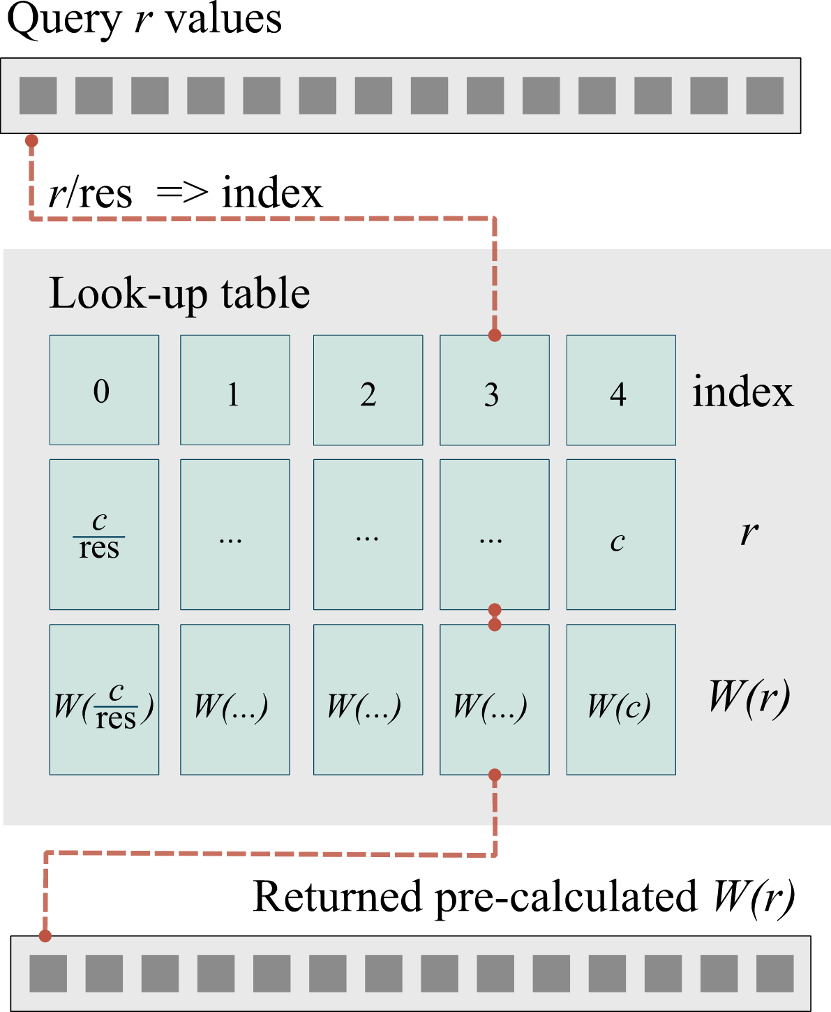
Example of a lookup table. Schematic diagram of the lookup table algorithm implemented in Pysammos. r corresponds to the distance between a particle and a grid point. The resolution of the lookup table is res. W(r) is the Coarse-Graining function, and c corresponds to its cut-off distance (i.e., *W(c)*=0).
This module provides functions to build and query hash tables for fast approximate evaluation of expensive functions. A hash table is constructed by precomputing function outputs at discrete input intervals. Queries on arbitrary inputs are answered by indexing into this table, trading some precision for speed.
- This module contains the following functions:
make_hash_table(): Constructs a hash table of function values by sampling a given function over a specified range.hash_table_search_1d(): Efficiently searches the hash table for 1D arrays of query values.hash_table_search_2d(): Efficiently searches the hash table for 2D arrays of query values.hash_table_search(): Dispatcher that routes queries to the correct 1D or 2D search function based on input dimensionality.
- pysammos.spatial_weights.hashtable_search.hash_table_search(query_values, hash_table_outputs, step_size)[source]
Dispatch function to route query_values to the appropriate hash table search function based on dimensionality.
Inputs
- query_valuesnp.ndarray
Input values to query. Must be 1D or 2D array.
- hash_table_outputsnp.ndarray
Precomputed hash table outputs.
- step_sizefloat
Sampling interval used in hash table construction.
Outputs
- np.ndarray
Approximated function values with same shape as query_values.
- raises ValueError:
If query_values is not 1D or 2D.
- pysammos.spatial_weights.hashtable_search.hash_table_search_1d(query_values, hash_table_outputs, step_size)
Approximate function evaluation for 1D query arrays by indexing into the precomputed hash table.
Inputs
- query_valuesnp.ndarray, shape (N,)
1D array of input values to query.
- hash_table_outputsnp.ndarray, shape (M,)
Precomputed function values stored in the hash table.
- step_sizefloat
Sampling interval used to build the hash table.
Outputs
- query_resultsnp.ndarray, shape (N,)
Approximated function values corresponding to each input query.
- pysammos.spatial_weights.hashtable_search.hash_table_search_2d(query_values, hash_table_outputs, step_size)
Approximate function evaluation for 2D query arrays by indexing into the precomputed hash table.
Inputs
- query_valuesnp.ndarray, shape (N, M)
2D array of input values to query.
- hash_table_outputsnp.ndarray, shape (K,)
Precomputed function values stored in the hash table.
- step_sizefloat
Sampling interval used to build the hash table.
Outputs
- outnp.ndarray, shape (N, M)
Approximated function values corresponding to each input query.
- pysammos.spatial_weights.hashtable_search.make_hash_table(func, max_value, sensitivity)[source]
Construct a hash table by sampling a function at discrete input intervals.
Inputs
- funccallable
The function to sample. Must accept two arguments: max_value and input_value.
- max_valuefloat
The maximum input value to sample up to.
- sensitivityfloat
Controls the granularity of the hash table sampling by dividing the position of the first significant digit of max_value.
Outputs
- hash_table_outputsnp.ndarray
Array of function values sampled at discrete points from step_size to max_value.
- step_sizefloat
The sampling interval between hash table inputs.
Notes
The step_size is calculated as the position of the first significant figure of max_value divided by sensitivity. The hash table inputs are then generated from step_size up to max_value in increments of step_size. The function is vectorized over these inputs to produce the outputs.
Kernels module
pysammos.spatial_weights.kernels module
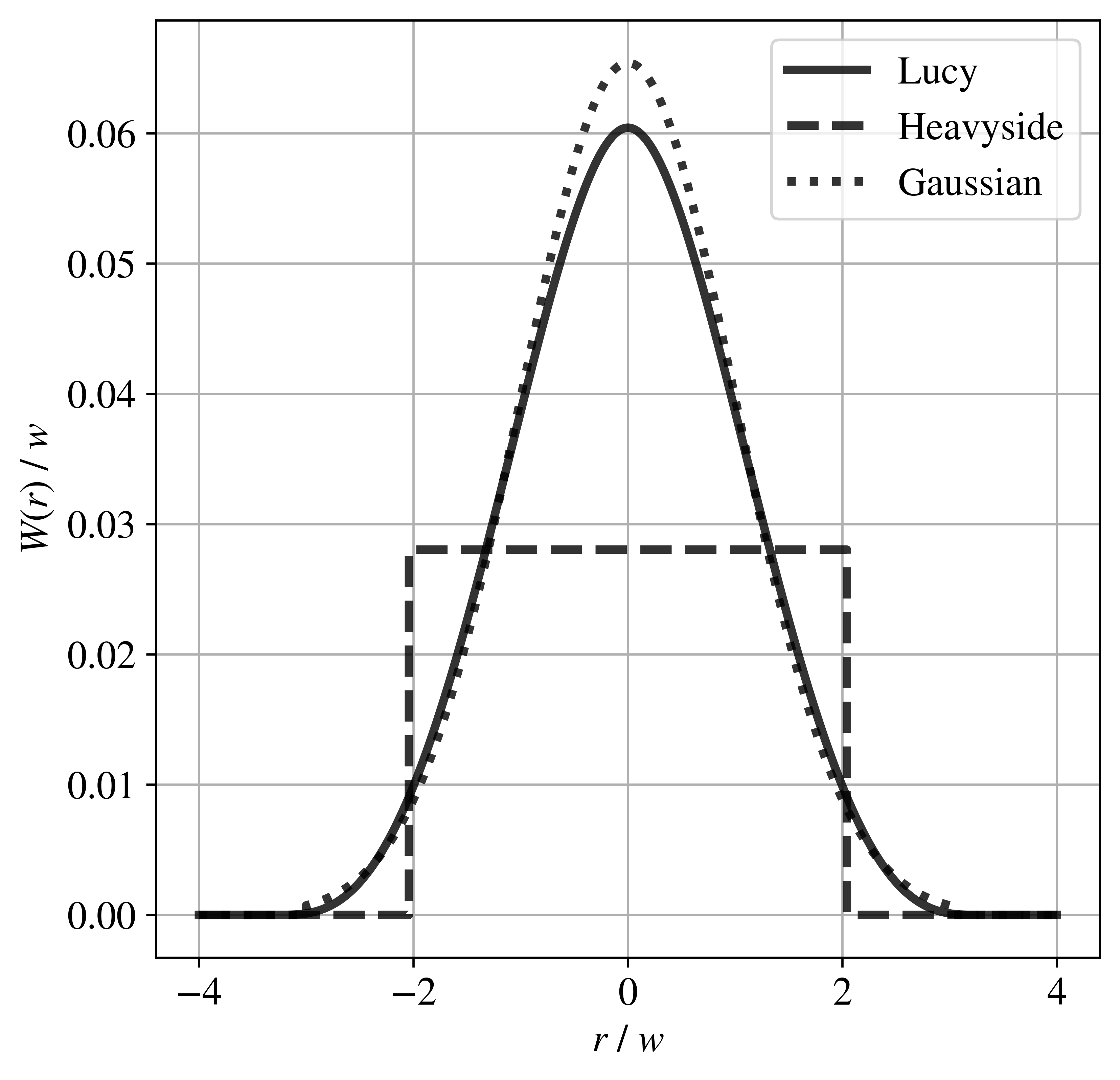
Example of spatial weights kernels. Visualisation of the three implemented Coarse-graining weighting functions, W(r), in one dimension (r) normalised by the half-width (w). Note that the functions have been plotted with equal variance in order to ensure that any differences are due to kernel shape, not scale.
This module provides a collection of commonly used kernel functions for smoothing, weighting, and interpolation in particle-based methods such as Smoothed Particle Hydrodynamics (SPH) or coarse-graining techniques.
This module includes implementations of several kernel functions:
lucy(): The Lucy kernel, a smooth, compactly supported kernel with continuous derivatives.
h(): The top-hat (step) function, a simple binary indicator function.
heavySide(): The Heaviside kernel, which provides uniform weighting inside a spherical cutoff volume.
gaussian(): The Gaussian kernel, a smooth, bell-shaped kernel with compact support truncated at three standard deviations.
Each kernel function computes a weight based on the distance from a kernel center and a cutoff radius, ensuring locality and normalization properties as appropriate.
- pysammos.spatial_weights.kernels.gaussian(c, dist)[source]
Gaussian kernel function with compact support.
Computes the Gaussian kernel value used for continuous interpolation or smoothing operations. The kernel is truncated at the cutoff distance c, which corresponds to three standard deviations.
\[w = \dfrac{c}{3}\]\[\begin{split}W(r) = \begin{cases} \dfrac{1}{V_w} \exp\left(-\dfrac{r^2}{2w^2}\right) & \text{if } r \leq c \\ 0 & \text{if } r > c \end{cases}\end{split}\]where \(V_w\) is a normalization constant to ensure the kernel integrates to 1:
\[V_w = 2\sqrt{2}w^3\pi^{3/2} \operatorname{erf}\left(\dfrac{c\sqrt{2}}{2w}\right) - 4cw^2\pi \exp\left(-\dfrac{c^2}{2w^2}\right)\]Inputs
- cfloat
Cutoff distance (typically 3σ).
- distfloat
Distance between the evaluation point and the kernel center.
Outputs
- Wfloat
The Gaussian kernel value.
- pysammos.spatial_weights.kernels.h(dis)[source]
Top-hat (step) function.
A basic step function defined as:
\[\begin{split}h(x) = \begin{cases} 1 & \text{if } x > 0 \\ 0 & \text{otherwise} \end{cases}\end{split}\]Inputs
- disfloat
Input value.
Outputs
- int
1 if dis > 0, otherwise 0.
- pysammos.spatial_weights.kernels.heavySide(c, dist)[source]
Heaviside kernel function.
Computes the Heaviside (uniform sphere) kernel value for a given distance.
The function returns:
\[\begin{split}H(r) = \begin{cases} \dfrac{1}{\Omega} & \text{if } r \leq c \\ 0 & \text{otherwise} \end{cases}\end{split}\]where \(\Omega = \dfrac{4}{3}\pi c^3\) is the normalization volume of a sphere.
Inputs
- cfloat
Cutoff distance (radius of the uniform sphere).
- distfloat
Distance from the kernel center.
Outputs
- HSfloat
The Heaviside kernel value.
- pysammos.spatial_weights.kernels.lucy(c, dist)[source]
Lucy kernel function.
Computes the Lucy weight at a given distance within the cutoff radius.
The Lucy kernel is defined as:
\[\begin{split}W(r) = \begin{cases} \dfrac{105}{16\pi c^3} \left( -3\left(\dfrac{r}{c}\right)^4 + 8\left(\dfrac{r}{c}\right)^3 - 6\left(\dfrac{r}{c}\right)^2 + 1 \right) & \text{if } r \leq c \\ 0 & \text{if } r > c \end{cases}\end{split}\]Inputs
- cfloat
Cutoff distance.
- distfloat
Distance between the evaluation point and the kernel center.
Outputs
- Wfloat
The weight computed from the Lucy kernel.
Resolution module
pysammos.spatial_weights.resolution module
This module provides helper functions for determining characteristic length scales used in kernel-based coarse-graining, smoothing, and interpolation methods. These parameters are essential in defining the support domain of a kernel function and thus controlling the spatial resolution of computed fields.
- This module includes the following functions:
calc_half_width(): Computes the kernel half-width w from an average particle diameter D scaled by a user-defined multiplicative factor.calc_cutoff(): Computes the kernel cutoff radius c based on the half-width w and the chosen kernel type (Lucy, Gaussian, or HeavySide).
These functions are often called during preprocessing to set consistent smoothing parameters for all particles in a simulation, ensuring that the kernel shape and support are appropriately scaled to particle size.
- pysammos.spatial_weights.resolution.calc_cutoff(w, function)[source]
Calculate the cutoff radius c for a given kernel function.
This function determines the cutoff distance \(c\) used to truncate the kernel or filter function, based on the half-width w and the specified kernel type.
The cutoff c is calculated as:
For the Lucy kernel: \(c = 2w\)
For the Gaussian kernel: \(c = 3w\)
For the Heaviside (step) function: \(c = w\)
Inputs
- wfloat
The half-width parameter used in the kernel.
- functionstr
The name of the kernel function. Must be one of: 'Lucy', 'Gaussian', or 'HeavySide'.
Outputs
- cfloat
The calculated cutoff value.
- raises ValueError:
If the function argument is not one of the supported types.
- pysammos.spatial_weights.resolution.calc_half_width(Average_part_diam, w_mult=0.75)[source]
Calculate the half-width parameter w based on average particle diameter.
This function computes the smoothing or weighting half-width w used in kernel functions for back-projection or filtering processes. The value of w is computed by scaling the average particle diameter by a multiplicative factor.
\[w = w_{\text{mult}} \cdot D\]where \(D\) is the average particle diameter and \(w_{\text{mult}}\) is the user-defined multiplicative scaling factor.
Inputs
- Average_part_diamfloat
The average particle diameter \(D\).
- w_multfloat, optional
The multiplicative factor for calculating the half-width w. Default is 0.75.
Outputs
- wfloat
The computed half-width w.
This module provides utility functions commonly used in numerical computations, particularly in physics and engineering simulations involving integration along branches or paths, and geometric distance calculations.
This module includes the following functions:
first_significant_figure_position(): Computes the positional value of the first significant figure in a given number.
integration_scalar(): Generates a linearly spaced scalar array for integration purposes.
trapezoidal_integration(): Performs trapezoidal numerical integration on a sampled function W over an interval.
compute_dist_along_branch(): Computes Euclidean distances along a branch for multiple contact points and scalar steps.
- pysammos.spatial_weights.utils.compute_dist_along_branch(r_ri_c, s, BranchVector_i, part_ind_c)
Compute Euclidean distances along a branch for multiple contact points and scalar steps.
\[d_{ij} = \left\| \mathbf{r}_{ri}^{(j)} + s_i \, \mathbf{B}_{\text{part}}^{(k_j)} \right\|_2\]where:
\(d_{ij}\) is the distance for scalar step \(s_i\) and contact point \(j\), \(\mathbf{r}_{ri}^{(j)}\) is the displacement vector from the reference point to contact point \(j\), \(s_i\) is the scalar step along the branch, \(\mathbf{B}_{\text{part}}^{(k_j)}\) is the branch direction vector associated with particle \(k_j\), and \(k_j = \text{part_ind_c}[j]\) is the index mapping contact points to particles.
Inputs
- r_ri_cnp.ndarray, shape (n_contacts, 3)
Displacement vectors from reference points to contact points.
- snp.ndarray, shape (n_s,)
Scalars along the branch for which distances are computed.
- BranchVector_inp.ndarray, shape (n_particles, 3)
Branch direction vectors associated with each particle.
- part_ind_cnp.ndarray, shape (n_contacts,)
Indices mapping contacts to corresponding particles in BranchVector_i.
Outputs
- np.ndarray, shape (n_s, n_contacts)
Euclidean distances along the branch for each scalar step and contact.
Notes
This function is JIT-compiled with Numba and parallelized for efficiency.
Examples
>>> r_ri_c = np.array([[1,0,0], [0,1,0]], dtype=np.float64)
>>> s = np.array([0, 1], dtype=np.float64)
>>> BranchVector_i = np.array([[1,0,0], [0,1,0]], dtype=np.float32)
>>> part_ind_c = np.array([0, 1], dtype=np.int32)
>>> compute_dist_along_branch(r_ri_c, s, BranchVector_i, part_ind_c)
array([[1., 1.],
       [2., 2.]])
- pysammos.spatial_weights.utils.first_significant_figure_position(number)[source]
Calculate the position (value) of the first significant figure of a number.
- Return type:
float
Inputs
- numberfloat
Input number to analyze.
Outputs
- float
The value of the first significant figure's position. For example, if number = 345.6, returns 100.0. Special case: returns 0 if number is zero.
Examples
>>> first_significant_figure_position(345.6)
100.0
>>> first_significant_figure_position(0.00789)
0.001
>>> first_significant_figure_position(0)
0
- pysammos.spatial_weights.utils.integration_scalar(s0, s1, n)[source]
Create a linearly spaced scalar array for integration over [s0, s1].
- Return type:
ndarray
Inputs
- s0float
Start of the integration interval.
- s1float
End of the integration interval.
- nint
Number of sample points.
Outputs
- np.ndarray, shape (n,)
Linearly spaced array of scalars from s0 to s1.
Examples
>>> integration_scalar(0, 1, 5)
array([0.  , 0.25, 0.5 , 0.75, 1.  ])
- pysammos.spatial_weights.utils.trapezoidal_integration(s0, s1, n, W)[source]
Compute numerical integral of sampled function W using the trapezoidal rule.
\[\begin{split}I_m = \int_{s_0}^{s_1} W_m(s) \, ds \approx \frac{\Delta s}{2} \left( W_m(s_0) + 2 \sum_{i=1}^{n-2} W_m(s_i) + W_m(s_{n-1}) \right) \\ \text{for } m = 0, \ldots, M-1\end{split}\]where: \(I_m\) is the integral of the m-th component of W, \(W_m(s)\) is the m-th component of the function W evaluated at s, \(s_0\) and \(s_1\) are the integration bounds, \(n\) is the number of sample points, \(\Delta s = \frac{s_1 - s_0}{n-1}\) is the step size, and \(M\) is the number of components (columns) in W.
Inputs
- s0float
Start of the integration interval.
- s1float
End of the integration interval.
- nint
Number of sample points.
- Wnp.ndarray, shape (n, m)
Values of the function sampled at the points defined by s0, s1, and n. Integration is performed along the first axis.
Outputs
- np.ndarray, shape (m,)
Resulting integral values for each column of W.
Examples
>>> s0, s1, n = 0, 1, 5
>>> W = np.array([[0], [1], [4], [9], [16]])
>>> trapezoidal_integration(s0, s1, n, W)
array([5.0])